Contents

Example: Spectral Analysis of a Whale Call

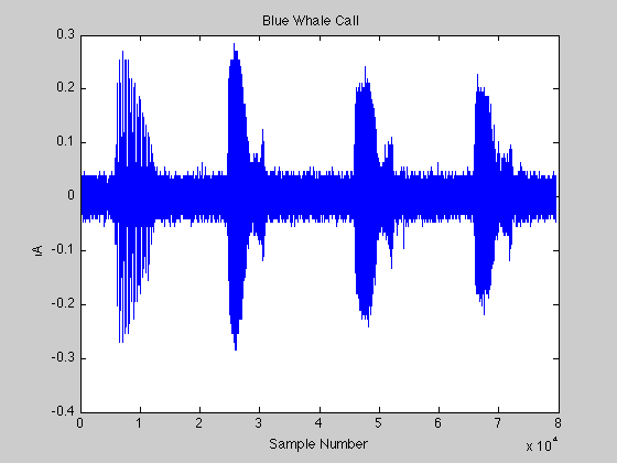
% The documentation example file bluewhale.au contains
% audio data from a Pacific blue whale vocalization
% recorded by underwater microphones off the coast of
% California. The file is from the library of animal
% vocalizations maintained by the Cornell University
% Bioacoustics Research Program.

% Because blue whale calls are so low, they are barely
% audible to humans. The time scale in the data is
% compressed by a factor of 10 to raise the pitch and
% make the call more clearly audible. The following
% reads, plots, and plays the data:

Loading sounds

[x,fs] = auread('BlueAtlx20.au');

[x,fs] = auread('BluePacx10.au');

figure
plot(x)
xlabel('Sample Number')
ylabel('Amplitude')
title('{\bf Blue Whale Call}')

sound(x,fs)

Plotting a signal's segment

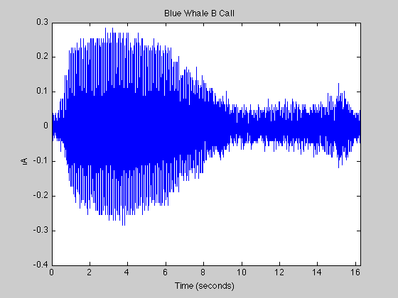
% An A "trill" is followed by a series of B "moans."

% The B call is simpler and easier to analyze.
% Use the previous plot to determine approximate
% indices for the beginning and end of the first
% B call. Correct the time base for the factor
% of 10 speed-up in the data:

bCall = x(2.45e4:3.10e4);
tb = 10*(0:1/fs:(length(bCall)-1)/fs); % Time base

figure
plot(tb,bCall)
xlim([0 tb(end)])
xlabel('Time (seconds)')
ylabel('Amplitude')
title('{\bf Blue Whale B Call}')

Impement FFT

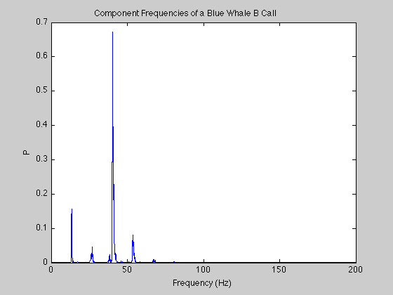
% Use fft to compute the DFT of the signal.
% Correct the frequency range for the factor of 10 speed-up in the data:

m = length(bCall);      % Window length
n = pow2(nextpow2(m));  % Transform length
y = fft(bCall);         % DFT of signal
f = (0:n-1)*(fs/n)/10;  % Frequency range
p = y.*conj(y)/n;       % Power of the DFT

% Plot the first half of the periodogram,
% up to the Nyquist frequency:

figure
plot(f(1:floor(n/2)),p(1:floor(n/2)))
xlabel('Frequency (Hz)')
ylabel('Power')
title('{\bf Component Frequencies of a Blue Whale B Call}')

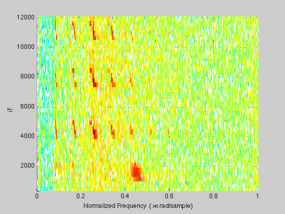
Spectrogram

figure
spectrogram(x,fs)

Published with MATLAB® 7.6