| Time series plot |
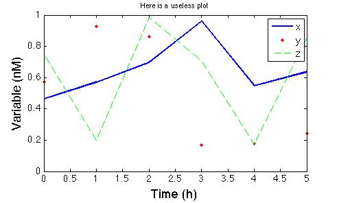 |
  T=[0:5]    % this generates a vecteur T with number 0 to 5
  D=rand(6)  % this generates a 6x6 matrix with random number between 0 and 1
  figure(1)
  set(figure(1),'Position', [400 400 500 300]);  % size of the figure
  clf;   % to clean the figure
  plot(T,D(:,2),'b',T,D(:,3),'r.',T,D(:,4),'g--');
  xlabel('Time (h)','fontsize',18);
  ylabel('Variable (nM)','fontsize',18);
  xlim([0 5]);
  ylim([0 1]);
  title('Here is a useless plot')
  legend('x','y','z');
  set(gca,'xtick',[0:0.5:6],'fontsize',14);
  set(findobj(gca,'Type','line','color','blue'),'LineWidth',2);
|
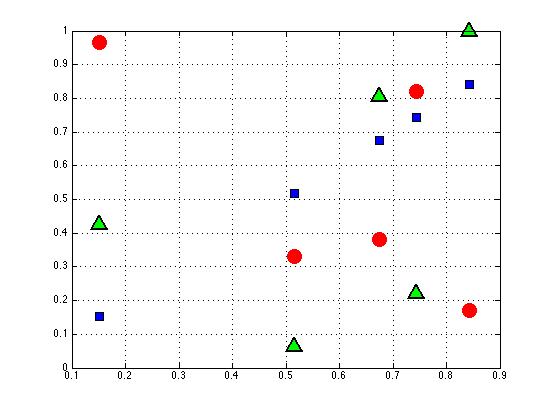
| Symbols plot |
 |
  figure(3)
  clf;
  T=[1:5];
  X=rand(5,1);
  Y=rand(5,1);
  Z=rand(5,1);
  plot(X,X,'rs','LineWidth',1,'MarkerEdgeColor','k','MarkerFaceColor','b','MarkerSize',10)
  hold on;
  plot(X,Y,'o','LineWidth',1,'MarkerEdgeColor','r','MarkerFaceColor','r','MarkerSize',15)
  hold on;
  plot(X,Z,'^','LineWidth',2,'MarkerEdgeColor','k','MarkerFaceColor','g','MarkerSize',15)
  Y=rand(5,1)
  grid on;
|
| Scatter plot |
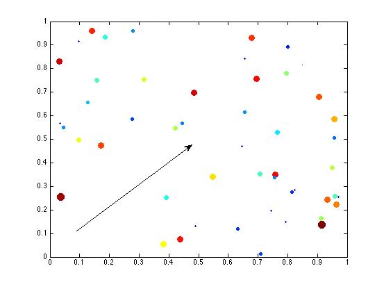 |
  N=50;    % number of points to generate
  X=rand(1,N);   % x-position
  Y=rand(1,N);   % y-position
  Z=rand(1,N);   % value (color) of the points
  %s=50;            % size of the points (same for all points)
  %s=100*rand(1,N); % size of the points (random)
  s=100*Z;          % size of the points (same vector as color)
  figure(1)
  clf;
  scatter(X,Y,s,Z,'filled')
  annotation('arrow',[0.2 0.5],[0.2 0.5])   % draw arrow
  box on;
|
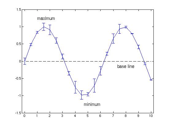
| Error bar |
 |
    figure(1)
    clf;
    x=[0:0.5:10];
    y=sin(x);
    e=rand(1,length(x))/5
    errorbar(x,y,e)
    hold on;
    plot([0 10],[0 0],'k--')
    text(8,-0.15,'base line','fontsize',14,'HorizontalAlignment','center');
    text(1,1.25,'maximum','fontsize',14,'HorizontalAlignment','left');
    text(6,-1.25,'minimum','fontsize',14,'HorizontalAlignment','right');
    xlim([-0.2 10.2]);
    ylim([-1.5 1.5]);
    box on;
|
| Double-y plot |
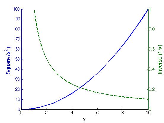 |
    figure(1);
    clf;

    x1=[0:0.5:10];
    y1=x1.^2;
    x2=[0.2:0.2:20];
    y2=1./x2;

    [AX,H1,H2]=plotyy(x1,y1,x2,y2);

    box off;
    set(get(AX(1),'Ylabel'),'String','Square (x^2)','fontsize',18)
    set(get(AX(2),'Ylabel'),'String','Inverse (1/x)','fontsize',18)
    set(H1,'LineWidth',2)
    set(H2,'LineWidth',2,'LineStyle','--')
    xlabel('x','fontsize',18);
    set(AX(1),'YLim',[0 100],'YTick',[0:10:100],'fontsize',15)
    set(AX(2),'YLim',[0 1],'YTick',[0:0.2:1],'fontsize',15)
    set(AX(1),'xlim',[0 10]);
    set(AX(2),'xlim',[0 10]);
|
| Bar plot |
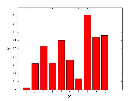 |
  figure(4)
  X=[1:10];
  Y=rand(10,1);
  bar(X,Y,'r');
  xlabel('X','fontsize',18);
  ylabel('Y','fontsize',18);
|
| Bar plot (multicolor) |
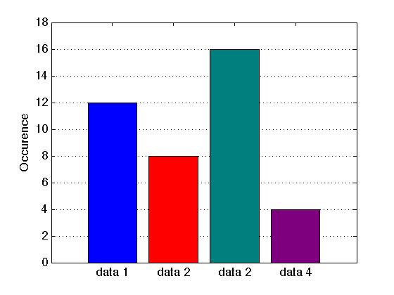 |
  D=[12 8 16 4];  % data

  figure(1)
  b=bar(1:4,D);   %  bar plot

  %%% trick to personnalize the color of each bar:
  ch=get(b,'children');
  cd=repmat(1:numel(D),5,1);
  cd=[cd(:);nan];
  set(ch,'facevertexcdata',cd);
  colormap([[0,0,1];[1,0,0];[0,0.5,0.5];[0.5,0,0.5]]);

  set(gca,'YGrid','on')  % horizontal grid

  ylim([0 max(D)+2]);

  set(gca,'XTickLabel',{'data 1','data 2','data 2','data 4'},'fontsize',14)
  ylabel('Occurence')
|
| Bar plot with error bars |
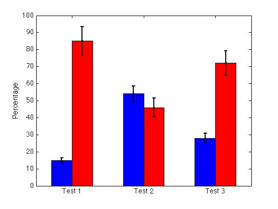 |
figure(1)

clf;

D=[15 85; 54 46; 28 72];       % data
S=[1.5 8.5; 4.6 5.4; 2.8 7.2]; % st dev (10%)

h=bar(D);
set(h,'BarWidth',1);
hold on;

ngroups = size(D,1);
nbars = size(D,2);
groupwidth = min(0.8, nbars/(nbars+1.5));

colormap([0 0 1; 1 0 0]);   % blue / red

for i = 1:nbars
x = (1:ngroups) - groupwidth/2 + (2*i-1) * groupwidth / (2*nbars);
errorbar(x,D(:,i),S(:,i),'k.','linewidth',2);
end

set(gca,'XTickLabel',{'Test 1','Test 2','Test 3'},'fontsize',14)
ylabel('Percentage','fontsize',14)
|
| Histogram |
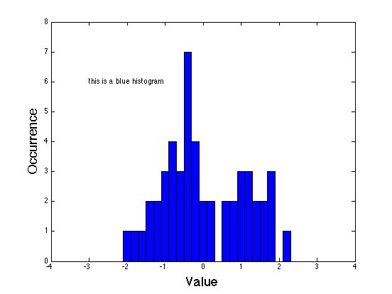 |
  D=randn(50,1)  % generates a vector with 50 numbers normally distributed
  figure(2)
  bin=[-4:0.2:4];
  hist(D,bin);
  xlabel('Value','fontsize',18);
  ylabel('Occurrence','fontsize',18);
  xlim([-4 4]);
  ylim([0 8]);
  set(findobj(gca,'Type','patch'),'FaceColor','b','EdgeColor','k')
  text(-3,6,'this is a blue histogram')
|
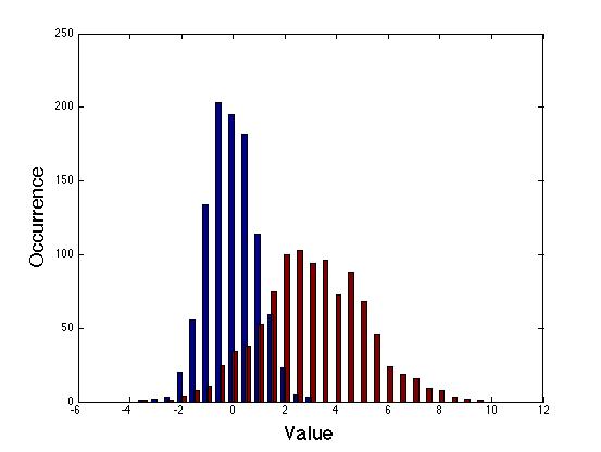
| Histogram with several populations |
 |
  figure(2)
  D1=randn(1000,1);  % generates a vector with 1000 random numbers normally distributed
  D2=2*randn(1000,1)+3; % generates a vector with 1000 random numbers normally distributed
  x=[-5:0.5:10];
  y1=hist(D1,x);
  y2=hist(D2,x);
  D=[y1; y2];
  bar(x,D',1.4);
  xlabel('Value','fontsize',18);
  ylabel('Occurrence','fontsize',18);
|
| Box plot |
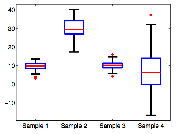 |
n=100;  % number of data points / sample

D(1:n,1)=10+2*randn(1,n);  % sample 1
D(1:n,2)=30+5*randn(1,n); % sample 2
D(1:n,3)=10+2*randn(1,n);  % sample 3
D(1:n,4)=5+10*randn(1,n); % sample 4

figure(1)
clf

h=boxplot(D,'plotstyle','traditional','whisker',1.5);

%%% Some alternatives:
% 'plotstyle'= 'compact' => useful of many boxes
% 'whisker'= 1.5 (default) => increased not to display outliers
% 'colors'='k' => plot in black

set(findobj(gcf,'LineStyle','--'),'LineStyle','-') % solid lines

for b=1:4 % loop on boxes
for i=1:size(h,1) % loop on the "elements" of a box
set(h(i,b),'linewidth',3);  % increase linewidth
end
end

mylabels={'Sample 1','Sample 2','Sample 3','Sample 4'};
mylabpos=[1:4];
set(gca,'XTickLabel',mylabels,'XTick',mylabpos,'fontsize',14);
|
| Fill polygons |
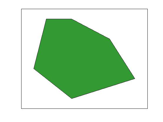 |
  x = [1 2 4 7 9 4];
  y = [4 9 9 7 3 1];
  col=[0.2 0.6 0.2]; % colour (RGB)
  fill(x,y,col);
  xlim([0 10]);
  ylim([0 10]);
  set(gca,'XTickLabel',{''})  % to remove x tick labels
  set(gca,'YTickLabel',{''})  % to remove y tick labels
  set(gca,'XTick',[])         % to remove x ticks
  set(gca,'YTick',[])         % to remove y ticks
  %axis off;                  % to remove the box
|
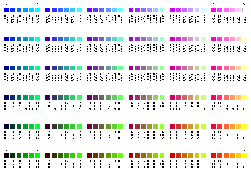
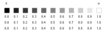
| Color map |
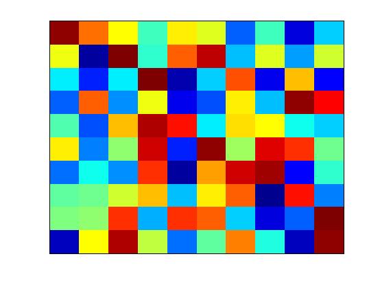 |
  X=rand(10);
  imagesc(X);
  colormap(jet);    % instead of 'jet' try 'gray', 'bone', 'spring',...
                    % >>help colormap for more color options.
  set(gca,'XTickLabel',{''})  % to remove x tick labels
  set(gca,'YTickLabel',{''})  % to remove y tick labels
  set(gca,'XTick',[])         % to remove x ticks
  set(gca,'YTick',[])         % to remove y ticks
|
| Pie chart |
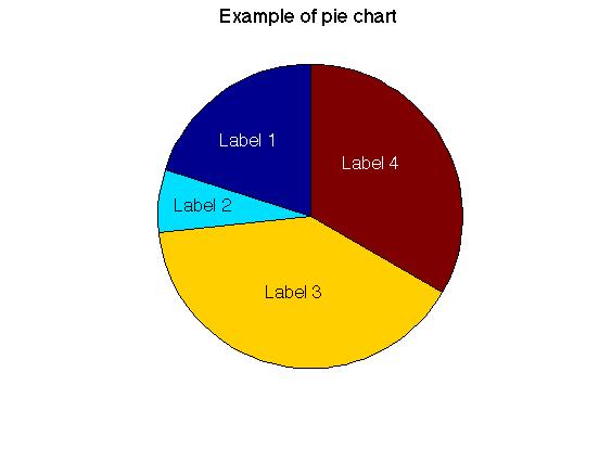 |
  x=[30 10 60 50];
  explode = [0 0 0 0];
  %explode = [0 2 0 0];
  labels = {'Label 1', 'Label 2', 'Label 3', 'Label 4'};
  %labels = [];     % to indicate percents instead of labels

  h=pie(x,explode,labels);   % try pie3 for 3D pie...
                             % NB: if no labels, the percentage are indicated.

  %set(h(2:2:8),'fontsize',16); % sise of the labels
  set(h(2),'fontsize',16,'position',[-0.4 0.5],'color','w');   % label 1
  set(h(4),'fontsize',16,'position',[-0.7 0.07],'color','k');  % label 2
  set(h(6),'fontsize',16,'position',[-0.1 -0.5],'color','k');  % label 3
  set(h(8),'fontsize',16,'position',[0.4 0.35],'color','w');   % label 4

  colormap jet
  %set(h(1),'facecolor','m');   % change color of piece 1 into magenta

  title('Example of pie chart','fontsize',18)
  %set(gca,'position',[0.13 0.11 0.775 0.815])  % to change plot position
  legend('lab1','lab2','lab3','lab4','location',[0.75 0.7 0.2 0.2])
|
| Plot 3D |
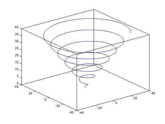 |
  figure(8)
  clf;

  x=[0:0.01:40];

  plot3(x.*sin(x),x.*cos(x),x,'b')

  box on;
|
| Surface |
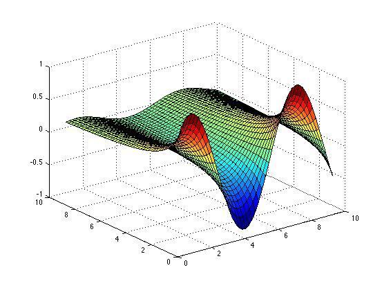 |
  x=[1:0.2:10];
  y=[1:0.2:10];

  for i=1:length(x)
  for j=1:length(y)
    z(i,j)=1./x(i).*sin(y(j));
  end
  end

  figure(2);
  clf;
  surf(x,y,z);
|
| Contour |
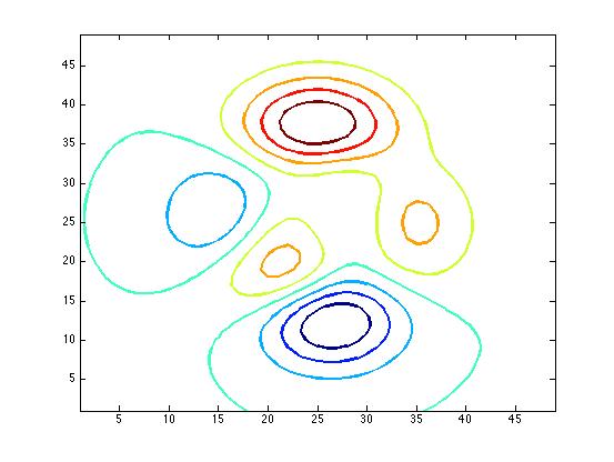 |
  z=peaks;  % demo data

  figure(2)
  clf;
  n=8; % number of contour plot (not mandatory)
  contour(z,n,'linewidth',2);

  %%% To write level on the contour lines:
  % [C,h]=contour(z,n,'linewidth',2)
  % set(h,'ShowText','on','TextStep',get(h,'LevelStep')*2)

  %%% Alternative representations:
  % contourf(z,n)   % to fill the regions between the contours
  % contour3(z,n)   % to draw the contours in 3D
|
| Surface + contour |
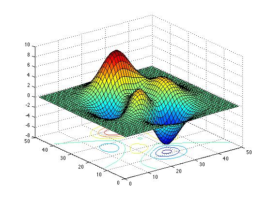 |
  z=peaks;  % demo data

  figure(4)
  clf;
  h=surfc(z);
  clev=-8;   % z-level of the contour lines
  for n=2:numel(h)
     z=get(h(n),'zdata');
     set(h(n),'zdata',ones(size(z))*clev); % Contours are draw at z=clev
  end
|
| Density |
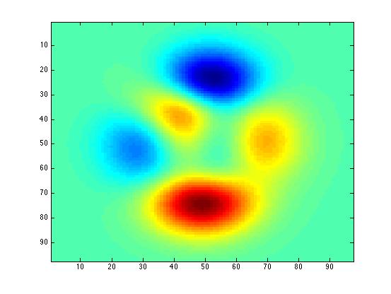 |
  z=peaks;  % demo data

  figure(3)
  clf;
  niter=1;
  method='bilinear';
  y=interp2(z,niter,method);
  imagesc(y);
|
| Geometrical shapes |
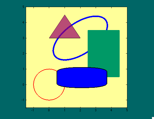 |
  %%% background colors

  whitebg([1.0 1.0 0.6])         % background color (in+out plot)
  set(gcf,'Color',[0,0.4,0.4])    % background color (out plot only)

  %%% circle

  circle = rsmak('circle');
  fnplt(circle)
  set(findobj(gca,'Color','blue'),'Color','r','LineWidth',2)

  xlim([-1.5 5])
  ylim([-1.5 5])
  axis square

  %%% ellipse

  hold on;
  S=[2,1];                                    % stretch
  T=[2;3];                                    % translation
  a=35*2*pi/360;                              % rotation angle
  R=[cos(a) sin(a);sin(a) -cos(a)];           % rotation matrix
  ellipse = fncmb(circle,[S(1) 0;0 S(2)]);    % stretch
  rtellipse = fncmb(fncmb(ellipse, R), T );   % rotate
  fnplt(rtellipse)
  set(findobj(gca,'Color','blue'),'Color','b','LineWidth',4)

  %%% rectangle

  hold on;
  c=[0.0 0.6 0.4];
  rectangle('Position',[2.5,0.5,2,3],'LineWidth',2,'facecolor',c,'edgecolor',c)

  %%% rounded rectangle

  hold on;
  rectangle('Position',[0.5,-0.2,3.2,1.3],'Curvature',[0.8,0.4],'LineWidth',2,'facecolor','b')

  %%% triangle

  hold on;
  h=patch([0 1 2], [3 4.5 3],'g');
  set(h,'facecolor',[0.6 0.0 0.4],'facealpha',0.7)
|
| Voronoi plot |
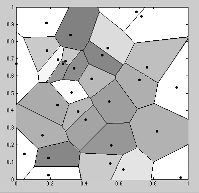 |
  N=30;  % number of cells

  x=rand(1,N);
  y=rand(1,N);

  D=[x;y]';

  [v,c]=voronoin(D);  % get edges

  for p=1:N

  r=rand()/2+0.5;    % color: random light grey
  col=[r r r];

  patch(v(c{p},1),v(c{p},2),col);  % color
  hold on;
  plot(x(p),y(p),'k.')        % dot at "center"

  end

  voronoi(x,y,'k')   % plot edges

  axis equal
  box on
  xlim([0 1])
  ylim([0 1])
|
| Sphere |
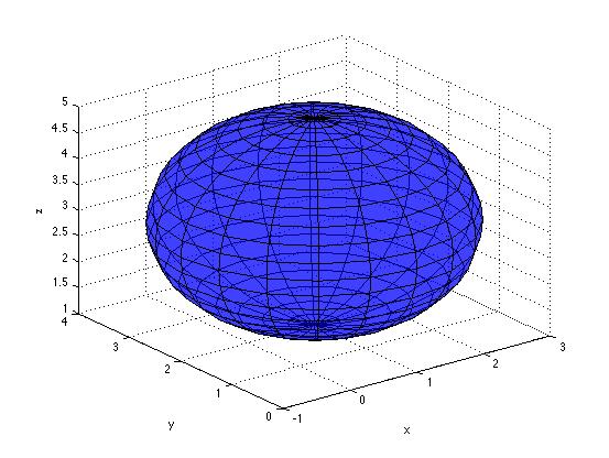 |
  r=20;               % resolution
  a=2;                % size of the sphere
  xc=1;yc=2;zc=3;     % coordinates of the center
  alpha=0.5;          % transparency

  [x,y,z]=sphere(r);

  figure(1)
  clf;

  surf(xc+x*a,yc+y*a,zc+z*a,'facecolor','blue','edgecolor','k','facealpha',alpha)
  %colormap('jet')   % colormap can be used if facecolor not used

  xlabel('x');
  ylabel('y');
  zlabel('z');
|
| Cube |
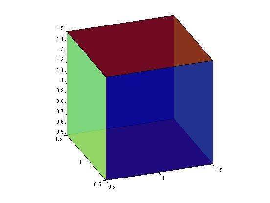 |
xc=1; yc=1; zc=1;    % coordinated of the center
L=1;                 % cube size (length of an edge)
alpha=0.8;           % transparency (max=1=opaque)

X = [0 0 0 0 0 1; 1 0 1 1 1 1; 1 0 1 1 1 1; 0 0 0 0 0 1];
Y = [0 0 0 0 1 0; 0 1 0 0 1 1; 0 1 1 1 1 1; 0 0 1 1 1 0];
Z = [0 0 1 0 0 0; 0 0 1 0 0 0; 1 1 1 0 1 1; 1 1 1 0 1 1];

% C='blue';                                                   % unicolor
C= [0.1 0.5 0.9 0.9 0.1 0.5];                                 % color/face
% C = [0.1 0.8 1.1 1.1 0.1 0.8 ; 0.2 0.9 1.2 1.2 0.2 0.8 ;
%      0.3 0.9 1.3 1.3 0.3 0.9 ; 0.4 0.9 1.4 1.4 0.4 0.9 ];   % color scale/face

X = L*(X-0.5) + xc;
Y = L*(Y-0.5) + yc;
Z = L*(Z-0.5) + zc;

fill3(X,Y,Z,C,'FaceAlpha',alpha);    % draw cube
axis equal;

AZ=-20;         % azimuth
EL=25;          % elevation
view(AZ,EL);    % orientation of the axes
|
| Multi-plot |
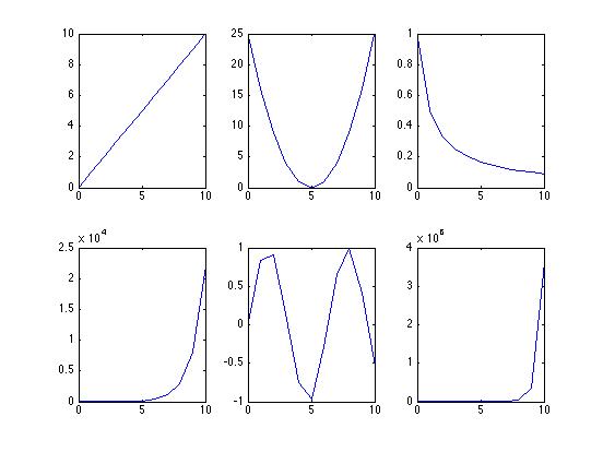 |
  figure(1)
  clf;

  x=[0:10];

  subplot(2,3,1)
  plot(x,x)

  subplot(2,3,2)
  plot(x,(x-5).^2)

  subplot(2,3,3)
  plot(x,1./(x+1))

  subplot(2,3,4)
  plot(x,exp(x))

  subplot(2,3,5)
  plot(x,sin(x))

  subplot(2,3,6)
  plot(x,factorial(x))
|
| Multi-plot |
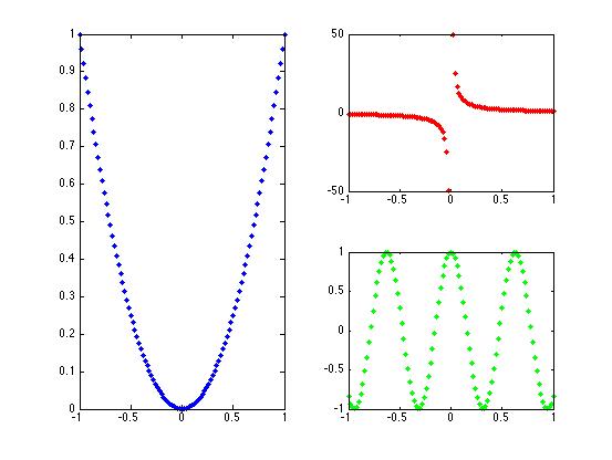 |
  figure(1)
  clf;

  x=[-1:0.02:1];

  subplot(2,2,[1 3])
  plot(x,x.^2,'b.')

  subplot(2,2,2)
  plot(x,1./x,'r.')

  subplot(2,2,4)
  plot(x,cos(10.*x),'g.')
|
| Multi-plot |
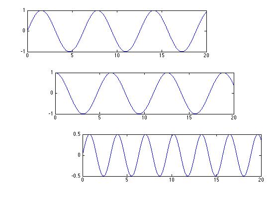 |
  figure(1)
  clf;

  x=[0:0.01:20];

  subplot('Position',[0.1 0.75 0.65 0.2])
  plot(x,sin(x),'b')

  subplot('Position',[0.2 0.45 0.65 0.2])
  plot(x,cos(x),'b')

  subplot('Position',[0.3 0.15 0.65 0.2])
  plot(x,sin(x).*cos(x),'b')
|
| Inset |
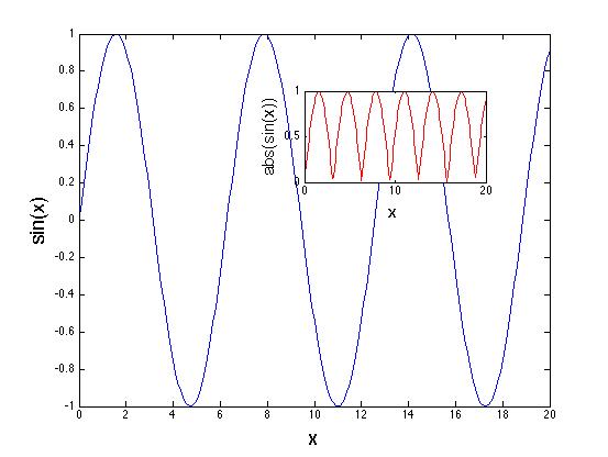 |
  figure(1)
  clf;

  x=[0:0.1:20]
  y=sin(x)

  subplot(1,1,1) ; % main plot

  plot(x,y,'b')
  xlabel('x','fontsize',18)
  ylabel('sin(x)','fontsize',18)

  axes('position',[0.5 0.6 0.3 0.2]) ; % inset

  plot(x,abs(y),'r')
  xlabel('x','fontsize',15)
  ylabel('abs(sin(x))','fontsize',15)
|
| |